Stochastic Models of the Social Security Trust Funds
Social Security Bulletin, Vol. 65, No. 1, 2003/2004
The 2003 Trustees Report on the Old-Age and Survivors Insurance and Disability Insurance Trust Funds contains, for the first time, results from a stochastic model of the combined trust funds of the OASDI programs. To help interpret the new stochastic results and place them in context, the Social Security Administration's Office of Policy arranged for three external modeling groups to produce alternative stochastic results. This article demonstrates that the stochastic models deliver broadly consistent results even though they use significantly different approaches and assumptions. However, the results also demonstrate that the variation in trust fund outcomes differs as the approach and assumptions are varied.
The authors are with the Division of Economic Research, Office of Research, Evaluation, and Statistics, Office of Policy, Social Security Administration. Eugene Bang, also with the Division of Economic Research, provided research assistance.
Acknowledgments: The authors thank all those who contributed results as well as David Pattison and John Sabelhaus for helpful conversations.
The findings and conclusions presented in the Bulletin are those of the authors and do not necessarily represent the views of the Social Security Administration.
NOTE: An earlier version of this article was published as Research and Statistics Note 2003-01, available at http://www.socialsecurity.gov/policy/docs/rsnotes/rsn2003-01.html.
Summary
Each year in March, the Board of Trustees of the Social Security trust funds reports on the current and projected financial condition of the Social Security programs. Those programs, which pay monthly benefits to retired workers and their families, to the survivors of deceased workers, and to disabled workers and their families, are financed through the Old-Age, Survivors, and Disability Insurance (OASDI) Trust Funds. In their 2003 report, the Trustees present, for the first time, results from a stochastic model of the combined OASDI trust funds.
Stochastic modeling is an important new tool for Social Security policy analysis and offers the promise of valuable new insights into the financial status of the OASDI trust funds and the effects of policy changes. The results presented in this article demonstrate that several stochastic models deliver broadly consistent results even though they use very different approaches and assumptions. However, they also show that the variation in trust fund outcomes differs as the approach and assumptions are varied. Which approach and assumptions are best suited for Social Security policy analysis remains an open question. Further research is needed before the promise of stochastic modeling is fully realized. For example, neither parameter uncertainty nor variability in ultimate assumption values is recognized explicitly in the analyses. Despite this caveat, stochastic modeling results are already shedding new light on the range and distribution of trust fund outcomes that might occur in the future.
Introduction
The stochastic model used in the 2003 Trustees Report was developed by the Office of the Chief Actuary (OCACT) of the Social Security Administration to illustrate the uncertainty surrounding projections of the financial future of the Social Security system over the next 75 years. The stochastic results are intended to augment the traditional demonstrations of uncertainty used in past Trustees Reports. The standard method of demonstrating uncertainty is to present three alternative sets of deterministic projections. The intermediate (Alternative II) projections are intended to reflect the best estimates of future experience. The low-cost (Alternative I) and high-cost (Alternative III) projections are based on more optimistic and more pessimistic assumptions about the future, respectively. The three alternatives indicate a possible range for future experience. The stochastic model also relies on the assumptions underlying the intermediate (Alternative II) projections. Time constraints dictated that the stochastic results in the 2003 Trustees Report be based on the assumptions from the 2002 report.
The purpose of stochastic modeling is to further illustrate the degree of uncertainty inherent in projecting future financial outcomes for the combined OASDI trust funds. Those outcomes depend on the future values of a large number of demographic, economic, and program-specific variables that cannot be known with certainty and must be forecast. Stochastic modeling is an attempt to forecast the future values of variables in a manner that is consistent with contemporary economic and demographic theory and with empirical evidence. The statistical techniques used in stochastic modeling help to ensure that the variables that determine the future financial condition of the combined OASDI trust funds evolve over time in a fashion that is consistent with their past behavior and is intended to be consistent with their actual future behavior. Simulation techniques are used to construct a large number of future financial outcomes for the trust funds. Each simulation makes random draws for the stochastic variables from their estimated probability distributions and uses those randomly drawn variables to produce future trust fund outcomes. The distribution of those simulated outcomes is then assumed to be representative of the range and distribution of actual outcomes that might be realized in the future.
To help interpret the new stochastic results and to place them in context, the Social Security Administration's Office of Policy arranged for three external modeling groups to produce alternative stochastic results that also used the assumptions from the 2002 Trustees Report.1 This article describes results produced by:
- The Congressional Budget Office Long Term (CBOLT) model;
- A model developed by Shripad Tuljapurkar and Ron Lee (TL), formerly of Mountain View Research; and
- The SSASIM model developed by the Policy Simulation Group.
The results from the three external models are analyzed and compared, with particular attention paid to the alternative assumptions and approaches adopted by each. The results are also compared with the stochastic results produced by OCACT and with the intermediate, high-cost, and low-cost projections traditionally used by the Trustees. The external models produce results that are quite similar to each other, but they do exhibit some differences when compared with both the stochastic and nonstochastic results produced by OCACT.
Highlights of the Models' Results
The major results from the models are summarized below and in Table 1.
| Model | Low range |
Intermediate range |
High range |
|---|---|---|---|
| Stochastic models | |||
| CBOLT | 2028 | 2037 | 2063 |
| TL | 2029 | 2037 | 2056 |
| SSASIM | a | 2037/2038 | a |
| OCACT | 2034 | 2041 | 2057 |
| Standard model (based on 2002 Trustees Report) | 2029 | 2041 | b |
| SOURCE: CBOLT = Congressional Budget Office Long Term Model; TL = model developed by Shripad Tuljapurkar and Ron Lee; OCACT = Office of the Chief Actuary. | |||
| NOTES: For the stochastic models, the low-, intermediate-, and high-range results are for the 10th, 50th, and 90th percentile, respectively. For the Trustees Report, the three ranges are for the high-cost, intermediate, and low-cost assumptions in the 2002 Trustees Report. | |||
| a. For this article, SSASIM modeled only two variables—productivity and fertility—stochastically, so the range of outcomes should not be compared with those of the other stochastic models. | |||
| b. According to the low-cost projections in the 2002 Trustees Report, the trust funds are not exhausted at the end of the 75-year projection period. | |||
CBOLT Model
The median simulation result from the CBOLT model projects that the combined OASDI trust funds will be exhausted in 2037—4 years earlier than the date of 2041 projected under the Alternative II assumptions in the 2002 Trustees Report. The CBOLT model projects a 10 percent chance that the trust funds will be exhausted by 2028, which is one year earlier than the Trustees' standard high-cost projection. The model also projects a 10 percent chance that exhaustion will not occur before 2063. In contrast, according to the Trustees' standard low-cost projection, the trust funds are not exhausted by 2076, the end of the 75-year projection period.
TL Model
The median simulation result from the TL model also projects exhaustion of the combined OASDI trust funds in 2037—again, 4 years earlier than projected by the standard model under the Alternative II assumptions in the 2002 Trustees Report. The TL model projects a 10 percent chance that the trust funds will be exhausted by 2029 and a 10 percent chance that exhaustion might not occur before 2056. These dates compare with the high-cost projection of 2029 and the low-cost projection from the 2002 Trustees Report that the trust funds will not be exhausted at the end of the 75-year projection period.
SSASIM Model
Although SSASIM is fully as capable as the other models, for this article it models only two variables stochastically—productivity and fertility. Therefore, the results from the SSASIM model shown here are not directly comparable with those of the other external models or with those produced by OCACT. Rather, the results are used to explore the implications of different modeling choices. The results show that stochastic modeling outcomes can exhibit significantly more variation when a structural time-series model is assumed than when an unrestricted reduced-form ARIMA model is used. (See box for an explanation of these two models.) The limited SSASIM model produces median simulation results that project exhaustion of the trust funds in 2037 and 2038 under the two different model specifications, respectively. Again, these dates are 3 to 4 years earlier than the date of 2041 projected under the intermediate assumptions in the 2002 Trustees' Report.
Structural and Unrestricted Reduced Form ARIMA Models
The relationships between variables that evolve over time are often described by a class of models known as ARIMA, for autoregressive integrated moving average. An ARIMA model represents the current value of variables as linear functions of their past values and of current and past values of random shocks to the system. ARIMA models are often used because they can capture the trends, cycles, and correlation patterns of most economic and demographic variables.
Because ARIMA models are so general, it is frequently necessary or desirable to impose additional restrictions on the model to rule out or impose certain types of behavior on the variables. When such restrictions are suggested by some theory or assumption, the model may be called structural. The restrictions of a structural model imply constraints on the coefficients of the models, and those constraints must be taken into account when the model is estimated.
When an ARIMA model is estimated without constraints, the model is called an unrestricted reduced form. An unrestricted reduced-form model seeks to capture the salient features of time-series relationships without any structure explaining how or why those relationships arise. Because unrestricted reduced-form models are estimated without any constraints imposed, they are usually easier to work with.
In the context of this article, the distinction between structural and reduced-form models arises because Holmer (2003) models some variables (the productivity growth rate and the total fertility rate) as the sum of a mean that varies over time and as a deviation from that mean that also varies over time. The structure that Holmer imposes places restrictions on the estimated coefficients of his model. These restrictions impose behavior on the variables that is consistent with the structure he assumes.
OCACT Model
Unlike the results of the three external models, the OCACT stochastic projections produce a median simulation result of trust fund exhaustion in 2041, the same as the standard Alternative II projection. The OCACT results indicate a 10 percent chance that the combined OASDI trust funds will be exhausted by 2034 and a 10 percent chance that they will not be exhausted before 2057.
All three external models produce median simulation results that project that the combined OASDI trust funds will be exhausted 3 to 4 years earlier than projected under Alternative II in the 2002 Trustees Report. By contrast, the OCACT median simulation results show trust fund exhaustion in the same year as Alternative II. Differences in the short-run behavior of the input variables and in the methodology used in modeling the long-run behavior of some variables may account for the divergent results, as explained below.
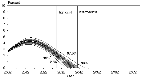
The trust fund ratio, or the ratio of trust fund assets at the beginning of the year to the year's expenditures, is a common measure of financial adequacy for the OASDI trust funds. The projections of the trust fund ratio from the CBOLT, TL, and OCACT stochastic models are detailed in the three fan charts shown in Chart 1. The projections from the SSASIM model are shown later because, for this article, the SSASIM model was restricted to modeling only two variables—productivity and fertility—stochastically, producing results that are not directly comparable with those of the other models.2
Trust fund ratio projections from the CBOLT, TL, and OCACT stochastic models
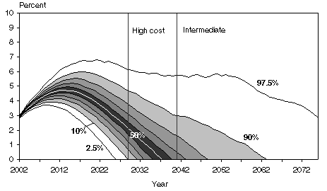
| 2.50% | 10% | 20% | 30% | 40% | 50% | 60% | 70% | 80% | 90% | 97.50% | |
|---|---|---|---|---|---|---|---|---|---|---|---|
| 2002 trust fund ratio | 2.81 | 2.84 | 2.86 | 2.88 | 2.90 | 2.91 | 2.92 | 2.94 | 2.95 | 2.97 | 3.00 |
| Peak trust fund ratio | 3.72 | 3.92 | 4.16 | 4.36 | 4.54 | 4.73 | 4.97 | 5.21 | 5.53 | 6.00 | 6.77 |
| Peak year | 2009 | 2011 | 2011 | 2012 | 2013 | 2013 | 2014 | 2015 | 2016 | 2018 | 2018 |
| Exhaustion year | 2025 | 2028 | 2031 | 2032 | 2034 | 2037 | 2039 | 2043 | 2048 | 2063 | a |
| a. The 97.5th percentile for the CBOLT model does not indicate trust fund exhaustion by 2076, the last year shown in the graph. The final trust fund ratio in that year is 2.84. | |||||||||||
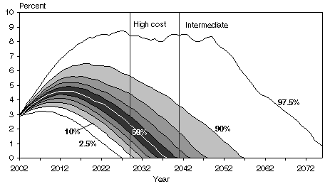
| 2.50% | 10% | 20% | 30% | 40% | 50% | 60% | 70% | 80% | 90% | 97.50% | |
|---|---|---|---|---|---|---|---|---|---|---|---|
| 2002 trust fund ratio | 2.71 | 2.71 | 2.71 | 2.71 | 2.71 | 2.71 | 2.71 | 2.71 | 2.71 | 2.71 | 2.71 |
| Peak trust fund ratio | 3.22 | 3.55 | 3.79 | 4.10 | 4.34 | 4.60 | 4.91 | 5.19 | 5.59 | 6.50 | 8.30 |
| Peak year | 2007 | 2010 | 2012 | 2012 | 2013 | 2014 | 2014 | 2016 | 2017 | 2018 | 2019 |
| Exhaustion year | 2026 | 2029 | 2031 | 2033 | 2035 | 2037 | 2040 | 2043 | 2047 | 2056 | a |
| a. The 97.5th percentile for the CBOLT model does not indicate trust fund exhaustion by 2076, the last year shown in the graph. The final trust fund ratio in that year is 0.85. | |||||||||||
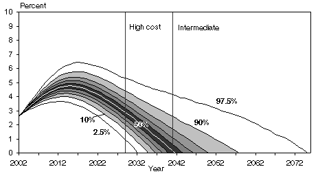
| 2.50% | 10% | 20% | 30% | 40% | 50% | 60% | 70% | 80% | 90% | 97.50% | |
|---|---|---|---|---|---|---|---|---|---|---|---|
| 2002 trust fund ratio | 2.60 | 2.60 | 2.60 | 2.60 | 2.61 | 2.61 | 2.61 | 2.61 | 2.61 | 2.61 | 2.61 |
| Peak trust fund ratio | 3.66 | 3.99 | 4.22 | 4.40 | 4.58 | 4.76 | 4.94 | 5.14 | 5.39 | 5.76 | 6.42 |
| Peak year | 2013 | 2013 | 2014 | 2015 | 2015 | 2015 | 2016 | 2015 | 2016 | 2017 | 2017 |
| Exhaustion year | 2032 | 2034 | 2036 | 2038 | 2039 | 2041 | 2043 | 2046 | 2050 | 2057 | 2075 |
The fan charts depict the 10th through the 90th percentiles of the simulation results. They also show the 2.5th and 97.5th percentiles. The percentiles do not represent individual simulation outcomes or paths. Rather, they describe the probability distribution of all of the simulation outcomes collectively. In each year, 10 percent of the simulated trust fund ratios fall below the 10th percentile, another 10 percent fall between the 10th and 20th percentiles, and so on. Finally, 10 percent of the simulated ratios for each year lie above the 90th percentile. Only 2.5 percent of the simulated ratios lie below the 2.5th percentile or above the 97.5th percentile. The fan charts are assumed to describe the probability distribution of future outcomes for the trust fund ratio that might be realized.
When the trust fund reaches zero, the combined OASDI trust funds are exhausted. Exhaustion dates shown in the fan charts match those in Table 1. In addition, the fan charts illustrate differences in how the various models depict the evolution of the trust funds over time.
Assumptions
The standard low-cost, intermediate, and high-cost projections described in the Trustees Report are each based on a set of assumptions for the variables that determine the financial future of the combined OASDI trust funds. Each set of assumptions consists of a short-range path and a long-range ultimate value for each variable. Those assumptions are agreed upon each year by the Trustees of the OASDI trust funds. The intermediate assumptions reflect the Trustees' best estimate for the future behavior of each variable. The new stochastic model developed by OCACT uses the intermediate assumptions to determine the mean, or expected value, of each of the stochastic variables.
The External Models
The external models also use the ultimate assumptions of Alternative II in the 2002 Trustees Report to determine the long-run expected value of the stochastic variables, with one exception. The TL model uses a method known as Lee-Carter to simulate future mortality. The Lee-Carter approach generates faster mortality improvement, resulting in longer life expectancies, than do the Trustees' 2002 intermediate assumptions about mortality.
The CBOLT and SSASIM methods for simulating future economic variables are similar to each other.3 Both models use a three-variable system of equations to simulate inflation, unemployment, and interest rates. The two models differ in that the CBOLT model simulates the real (inflation-adjusted) interest rate, while the SSASIM model simulates nominal interest rates. In addition, the CBOLT model adds an equation describing real wage growth, while the SSASIM model adds an equation for productivity growth. In contrast, the TL model adopts a different, reduced-form approach, modeling the real interest rate and the rate of real wage growth in separate equations and focusing on the effective real per capita tax rate without modeling unemployment and inflation directly.4
Despite their different approaches, the CBOLT and TL models produce stochastic projections that are broadly similar. The median results of both models project the same date of 2037 for trust fund exhaustion, 4 years sooner than projected under Alternative II in the 2002 Trustees Report. The SSASIM model produces median trust fund exhaustion dates of 2037 and 2038 for the two different model specifications considered. Again, these dates are 3 to 4 years earlier than projected under the Alternative II assumptions from the 2002 Report.
The OCACT Model
The assumptions regarding the behavior of stochastic variables in the OCACT model differ somewhat from those of the external models. The expected values of OCACT's input variables are calibrated to the Alternative II short-range assumptions for up to 25 years before settling into the Alternative II ultimate values (the CBOLT model also follows this approach). In addition, whereas in some cases the OCACT model projects the level of a variable, the external models project a nonlinear function (for example, the logarithm of the variable). In the external models, those projected nonlinear functions lead to asymmetric responses to shocks, which cause the median projections of the trust fund ratio to lie below the Alternative II projection. Because the procedure used to calibrate the stochastic simulations to the intermediate assumptions differs between the various models, the median projection results also differ.
Modeling Approaches Examined in the SSASIM Model
As mentioned above, the results from the SSASIM model are not directly comparable with those of the CBOLT and TL models. The SSASIM results do, however, highlight the importance of basic approaches when modeling the OASDI trust funds stochastically.
The model generates two sets of results, using two different specifications for the behavior of the stochastic variables. The results indicate greater dispersion of outcomes when a structural time-series specification is assumed for the stochastic variables. The structural time-series approach allows the behavior of stochastic variables to change over time. An unrestricted reduced-form ARIMA specification for the stochastic variables tends to produce less dispersion of outcomes. The structural time-series approach may produce a better fit to the historical data for some variables according to Holmer (2003). The trust fund ratio projections from the SSASIM model under both approaches are shown in Chart 2.
Comparison of trust fund ratio projections from the SSASIM model
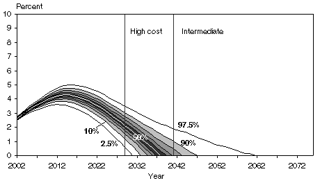
| 2.50% | 10% | 20% | 30% | 40% | 50% | 60% | 70% | 80% | 90% | 97.50% | |
|---|---|---|---|---|---|---|---|---|---|---|---|
| 2002 trust fund ratio | 2.51 | 2.55 | 2.58 | 2.59 | 2.61 | 2.62 | 2.64 | 2.65 | 2.67 | 2.70 | 2.73 |
| Peak trust fund ratio | 3.61 | 3.84 | 4.00 | 4.11 | 4.20 | 4.29 | 4.38 | 4.47 | 4.60 | 4.77 | 5.01 |
| Peak year | 2012 | 2013 | 2014 | 2014 | 2014 | 2015 | 2015 | 2015 | 2015 | 2015 | 2016 |
| Exhaustion year | 2030 | 2033 | 2034 | 2035 | 2036 | 2037 | 2039 | 2040 | 2043 | 2046 | 2061 |
| 2.50% | 10% | 20% | 30% | 40% | 50% | 60% | 70% | 80% | 90% | 97.50% | |
|---|---|---|---|---|---|---|---|---|---|---|---|
| 2002 trust fund ratio | 2.50 | 2.54 | 2.57 | 2.59 | 2.61 | 2.62 | 2.64 | 2.66 | 2.68 | 2.70 | 2.75 |
| Peak trust fund ratio | 3.76 | 3.95 | 4.08 | 4.16 | 4.23 | 4.31 | 4.37 | 4.46 | 4.55 | 4.66 | 4.87 |
| Peak year | 2014 | 2014 | 2014 | 2014 | 2014 | 2014 | 2015 | 2015 | 2014 | 2015 | 2015 |
| Exhaustion year | 2034 | 2035 | 2036 | 2037 | 2037 | 2038 | 2038 | 2039 | 2040 | 2042 | 2045 |
Additional Modeling Issues
The results from the three external models differ because of the varying approaches they adopt and the various assumptions each model makes. However, all three models have been carefully calibrated so that in the long run the expected values of stochastic variables, with the exception of mortality in the TL model, are in accord with the Alternative II assumptions from the 2002 Trustees Report. Hence, the results are conditional on the Alternative II assumptions. To eliminate this strict reliance on those assumptions, the ultimate rates to which the stochastic variables are calibrated can themselves be treated stochastically. Incorporating stochastic ultimate rates will add an additional dimension of uncertainty to the models, resulting in greater dispersion of the trust fund outcomes (Holmer 2003).
Yet another dimension of uncertainty concerns the parameter values used in the simulation of future values of the stochastic variables. Each of the models estimates its time-series equations using historical data. Once estimated, the coefficients are treated as if they are known with certainty. However, an alternative statistical approach would treat these estimated coefficients themselves as random, adding additional uncertainty to the stochastic models and resulting in still greater dispersion of the trust fund outcomes (Lee and Carter 1992).
Notes
1. An earlier version of the CBOLT model was documented in Congressional Budget Office (2001). Results from the TL model are documented in Lee, Anderson, and Tuljapurkar (2003). Those from the SSASIM model are described in Holmer (2003).
2. Previous results from the SSASIM model (Holmer 2002) that exploit its full stochastic capabilities have produced projections that are broadly similar to those of the CBOLT and TL models in all respects.
3. For this article, the SSASIM model was restricted to modeling only two variables—productivity and fertility—stochastically. Nevertheless, the SSASIM model has the ability to model all of the major trust fund determinants stochastically and is fully as capable as the other models described in this article. It is these more general capabilities that are referred to here.
4. The TL modeling team chose this approach after finding statistical evidence that the real interest rate and real wage growth are independent.
References
Board of Trustees of the Federal Old-Age and Survivors Insurance and Disability Insurance Trust Funds. 2002. 2002 Annual Report. Washington, D.C.: U.S. Government Printing Office. March. Available at http://www.socialsecurity.gov/OACT/TR/TR02/index.html.
__________. 2003. 2003 Annual Report. Washington, D.C.: U.S. Government Printing Office. March. Available at http://www.socialsecurity.gov/OACT/TR/TR03/index.html.
Congressional Budget Office. 2001. Uncertainty in Social Security's Long-Term Finances: A Stochastic Analysis. Technical Report. December. Available at http://www.cbo.gov.
Holmer, Martin R. 2002. Presentation to Office of Policy, Social Security Administration, Washington, D.C. June.
__________. 2003. Methods for Stochastic Trust Fund Projection. Report prepared for the Social Security Administration. January. Available at http://www.polsim.com/stochsim.pdf.
Lee, Ronald D., and Lawrence Carter. 1992. "Modeling and Forecasting the Time Series of U.S. Mortality." Journal of the American Statistical Association 87(419): 659–671.
Lee, Ronald D.; Michael W. Anderson; and Shripad Tuljapurkar. 2003. Stochastic Forecasts of the Social Security Trust Fund. Report prepared for the Social Security Administration. January.